Machine learning models learn from data and make predictions. One of the fundamental concepts behind training these models is backpropagation. In this article, we will explore what Backpropagation and Two Layer Back-Propagation Neural Network is, why it is crucial in machine learning, and how it works.

• Table of Content

1. Introduction

2. What is Backpropagation?

3. Why we need Backpropagation?

4. How Backpropagation algorithm works

5. Two type of working of Backpropagation algorithm

6. Example of two layer Backpropagation

7. Summary

Introduction

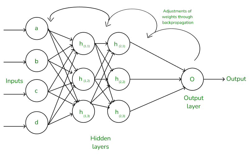
A Two layer Backpropagation Neural Network, also known as a Multilayer Perceptron (MLP), consists of an input layer, a hidden layer, and an output layer. The term "two-layer" refers to the presence of one hidden layer between the input and output layers.

Each layer contains multiple neurons (also known as nodes), and each neuron in one layer is connected to every neuron in the subsequent layer. These connections are associated with weights, which determine the strength of the connection between neurons. Shown below a simple illustration of Two layer backpropagation. (with hidden layer)

A neural network is a network structure, by the presence of computing units(neurons) the neural network has gained the ability to compute the function. The neurons are connected with the help of edges, and it is said to have an assigned activation function and also contains the adjustable parameters. These adjustable parameters help the neural network to determine the function that needs to be computed by the network. In terms of activation function in neural networks the higher the activation value is the greater the activation is.

What is Backpropagation?

• In machine learning, backpropagation is an effective algorithm used to train artificial neural networks, especially in feed-forward neural networks.

• Backpropagation is an iterative algorithm, that helps to minimize the cost function by determining which weights and biases should be adjusted. During every epoch, the model learns by adapting the weights and biases to minimize the loss by moving down toward the gradient of the error. Thus, it involves the two most popular optimization algorithms, such as gradient descent or stochastic gradient descent.

• Computing the gradient in the backpropagation algorithm helps to minimize the cost function and it can be implemented by using the mathematical rule called chain rule from calculus to navigate through complex layers of the neural network.

  

  Why We Need Backpropagation?

  Most prominent advantages of Backpropagation are:

  • Backpropagation is fast, simple and easy to program

  • It has no parameters to tune apart from the numbers of input

  • It is a flexible method as it does not require prior knowledge about the network

  • It is a standard method that generally works well

  • It does not need any special mention of the features of the function to be learned.

How Backpropagation Algorithm Works

• The Back propagation algorithm in neural network computes the gradient of the loss function for a single weight by the chain rule. It efficiently computes one layer at a time, unlike a native direct computation. It computes the gradient, but it does not define how the gradient is used. It generalizes the computation in the delta rule.

  Consider the following Back propagation neural network example diagram to understand:

  

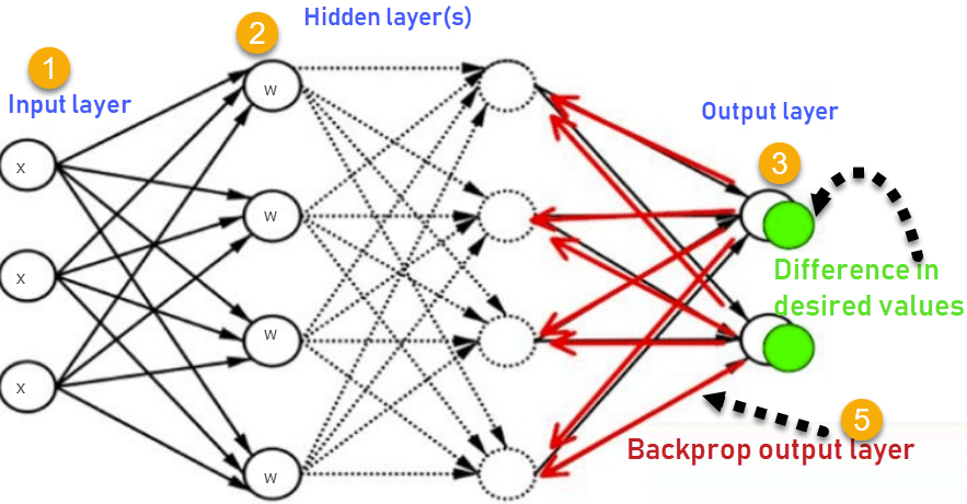
  How Backpropagation Algorithm Works

  1. Inputs X, arrive through the preconnected path

  2. Input is modeled using real weights W. The weights are usually randomly selected.

  3. Calculate the output for every neuron from the input layer, to the hidden layers, to the output layer.

  4. Calculate the error in the outputs

    ErrorB= Actual Output – Desired Output

5. Travel back from the output layer to the hidden layer to adjust the weights such that the error is decreased.

Working of Backpropagation Algorithm

The Backpropagation algorithm works by two different passes, they are:

• Forward pass

• Backward pass

How does Forward pass work?

• In forward pass, initially the input is fed into the input layer. Since the inputs are raw data, they can be used for training our neural network.

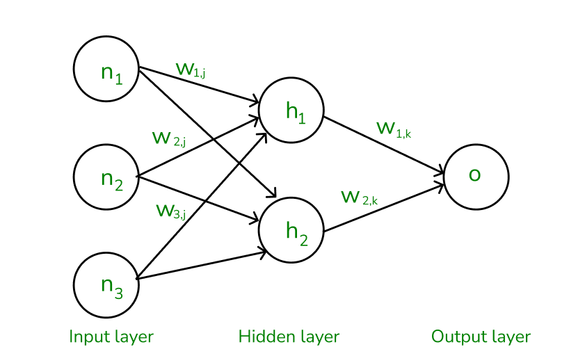
• The inputs and their corresponding weights are passed to the hidden layer. The hidden layer performs the computation on the data it receives. If there are two hidden layers in the neural network, for instance, consider the illustration fig(a), h₁ and h₂ are the two hidden layers, and the output of h₁ can be used as an input of h₂. Before applying it to the activation function, the bias is added.

• To the weighted sum of inputs, the activation function is applied in the hidden layer to each of its neurons. One such activation function that is commonly used is ReLU can also be used, which is responsible for returning the input if it is positive otherwise it returns zero. By doing this so, it introduces the non-linearity to our model, which enables the network to learn the complex relationships in the data. And finally, the weighted outputs from the last hidden layer are fed into the output to compute the final prediction, this layer can also use the activation function called the softmax function which is responsible for converting the weighted outputs into probabilities for each class.

How does backward pass work?

• In the backward pass process shows, the error is transmitted back to the network which helps the network, to improve its performance by learning and adjusting the internal weights.

• To find the error generated through the process of forward pass, we can use one of the most commonly used methods called mean squared error which calculates the difference between the predicted output and desired output. The formula for mean squared error is: Meansquarederror\=(predictedoutput–actualoutput)^2

• Once we have done the calculation at the output layer, we then propagate the error backward through the network, layer by layer.

• The key calculation during the backward pass is determining the gradients for each weight and bias in the network. This gradient is responsible for telling us how much each weight/bias should be adjusted to minimize the error in the next forward pass. The chain rule is used iteratively to calculate this gradient efficiently.

• In addition to gradient calculation, the activation function also plays a crucial role in backpropagation, it works by calculating the gradients with the help of the derivative of the activation function.

Example of Backpropagation

Let us now take an example to explain backpropagation,

Assume that the neurons have the sigmoid activation function to perform forward and backward pass on the network. And also assume that the actual output of y is 0.5 and the learning rate is 1. Now perform the backpropagation using backpropagation algorithm.

Implementing forward propagation:

Step1: Before proceeding to calculating forward propagation, we need to know the two formulae:

aj​=∑(wi​,j∗xi​)

Where,

• a_j is the weighted sum of all the inputs and weights at each node,

• wi,j – represents the weights associated with the j^th input to the i^th neuron,

• x_i – represents the value of the j^th input,

yj​=F(aj​)=1/1+e^−aj1, y_i – is the output value, F denotes the activation function [sigmoid activation function is used here), which transforms the weighted sum into the output value.

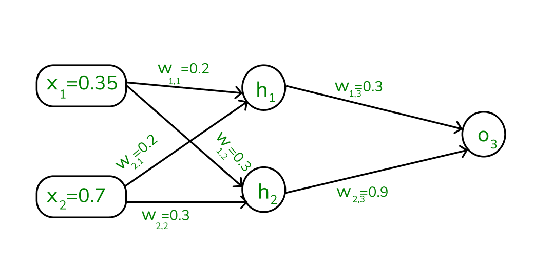
Step 2: To compute the forward pass, we need to compute the output for y₃ , y₄ , and y₅.

We start by calculating the weights and inputs by using the formula:

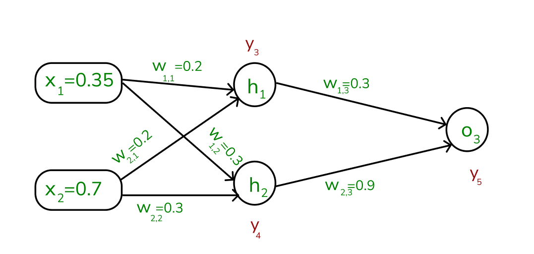
aj​=∑(wi,j​∗xi​) To find y₃ , we need to consider its incoming edges along with its weight and input. Here the incoming edges are from X₁ and X₂.

At h1 node,

a1​​=(w1,1​x1​)+(w2,1​x2​)=(0.2∗0.35)+(0.3∗0.7)=0.28​

Once, we calculated the a₁ value, we can now proceed to find the y₃ value:

yj​=F(aj​)=1/1+e^−aj1

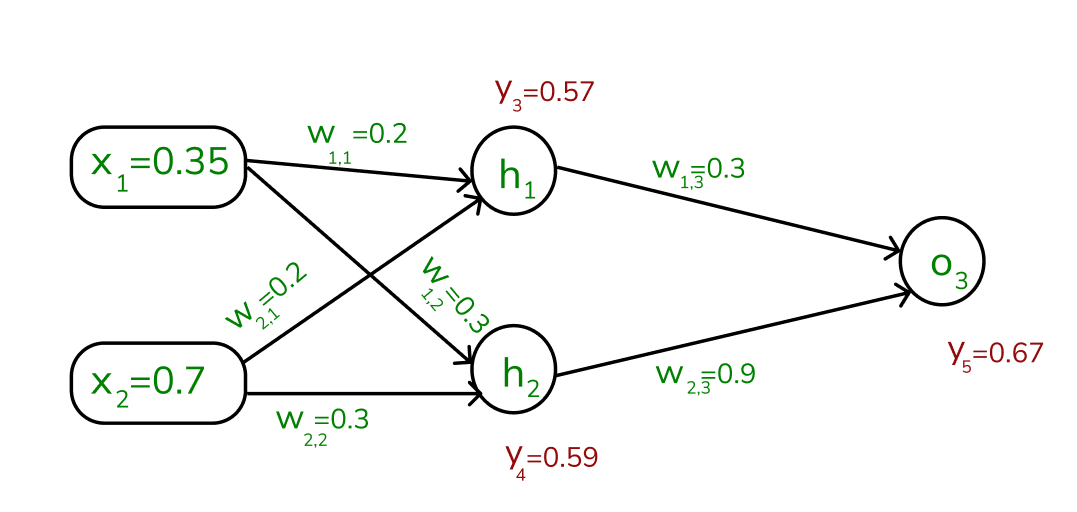
y3​=F(0.28)=1/1+e^−0.281​

y3​=0.57

Similarly find the values of y₄ at h₂ and y₅ at O_{3 ,}

a2=(w1,2​∗x1​)+(w2,2​∗x2​)=(0.3∗0.35)+(0.3∗0.7)=0.315

y4​=F(0.315)=1/1+e^−0.3151​

a3=(w1,3​∗y3​)+(w2,3​∗y4​)=(0.3∗0.57)+(0.9∗0.59)=0.702

y5​=F(0.702)=1/1+e^−0.7021​=0.67

Note that, our actual output is 0.5 but we obtained 0.67. To calculate the error, we can use the below formula:

Errorj​=ytarget​–y5​
Error = 0.5 – 0.67= -0.17

Using this error value, we will be backpropagating.

Implementing Backward Propagation

Each weight in the network is changed by,

∇wij = η 𝛿j Oj
𝛿j = Oj (1-Oj)(tj - Oj) (if j is an output unit)
𝛿j = Oj (1-O)∑k 𝛿k wkj (if j is a hidden unit)  
where ,
η is the constant which is considered as learning rate,

tj is the correct output for unit j

𝛿j is the error measure for unit j

Step 3: To calculate the backpropagation, we need to start from the output unit:

To compute the 𝛿₅, we need to use the output of forward pass,

𝛿₅ = y₅(1-y₅) (y_target -y₅)

\= 0.67(1-0.67) (-0.17)

\= -0.0376

For hidden unit,

To compute the hidden unit, we will take the value of 𝛿₅

𝛿₃ = y₃(1-y₃) (w_1,3 * 𝛿₅)

\=0.57(1-0.57) (0.3*-0.0375)

\=-0.0027

𝛿₄ = y₄ (1-y₅) (w_2,3 * 𝛿₅)

\=0.59(1-0.59) (0.9*-0.376)

\=-0.0819

Step 4: We need to update the weights, from output unit to hidden unit,

∇ wj,i = η 𝛿j Oj

Nte- Here our learning rate is 1

∇ w_2,3 = η 𝛿₅ O₄

\= 1 * (-0.376) * 0.59

\= -0.22184

We will be updating the weights based on the old weight of the network,

w_2,3(new) = ∇ w_4,5 + w_4,5 (old)

\= -0.22184 + 0.9

\= 0.67816

From hidden unit to input unit,

For an hidden to input node, we need to do calculations by the following;

∇ w_1,1 = η 𝛿₃ O₄

\= 1 (-0.0027) 0.35

\= 0.000945

Similarly, we need to calculate the new weight value using the old one:

w_1,1(new) = ∇ w_1,1+ w_1,1 (old)

\= 0.000945 + 0.2

\= 0.200945

Similarly, we update the weights of the other neurons: The new weights are mentioned below

w_1,2 (new) = 0.271335

w_1,3 (new) = 0.08567

w_2,1 (new) = 0.29811

w_2,2 (new) = 0.24267

The updated weights are illustrated below,

Once, the above process is done, we again perform the forward pass to find if we obtain the actual output as 0.5.

While performing the forward pass again, we obtain the following values:

y₃ \= 0.57

y₄ = 0.56

y₅ = 0.61

We can clearly see that our y₅ value is 0.61 which is not an expected actual output, So again we need to find the error and backpropagate through the network by updating the weights until the actual output is obtained.

Error \= ytarget​–y5​
\= 0.5 – 0.61 = -0.11

This is how the Two layer backpropagate works, it will be performing the forward pass first to see if we obtain the actual output, if not we will be finding the error rate and then backpropagating backwards through the layers in the network by adjusting the weights according to the error rate. This process is said to be continued until the actual output is gained by the neural network.

• References:

• Tom M. Mitchell (2017) McGraw-Hill Science/Engineering/Math; "Machine Learning"; First Edition ISBN: 0070428077

• Nielsen, Michael A.(2015). "How the backpropagation algorithm works"

• Images: https://www.geeksforgeeks.org/